That Brother laser printer you bought can also pretend it’s a plotter. One of the requirements embedded in a PCL-compatible printer is an implementation of HP-GL/2. This is a slightly modified version of the page description language used by HP’s pen plotters. With care, you can make proofs on a laser printer.
But add some magic header bytes (0x1b, 0x45, 0x1b, 0x25, 0x30, 0x42) and some trailer bytes (0x1b, 0x25, 0x30, 0x41, 0x1b, 0x45), and your printer understands it’s a PCL file.
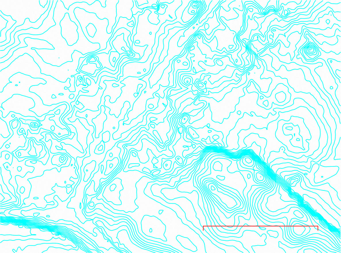
The file, complete with header and trailer, is here:
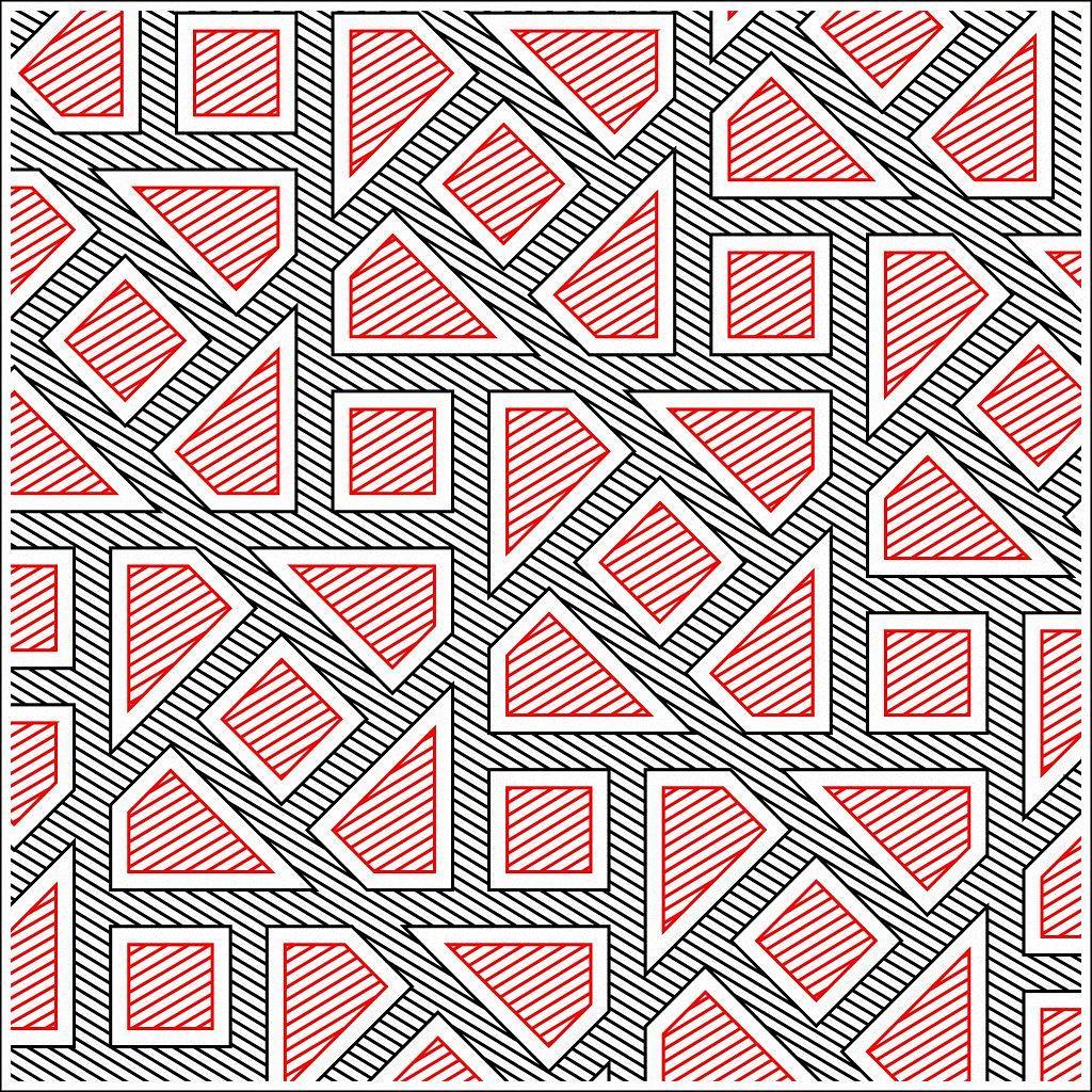
full page scan of that HP-GL file as printed on a Brother MFC-L2750DW
HP-GL/2, on mono lasers at least, has some differences to the version used on plotters. The biggest difference is that there’s just one pen. You can change the pattern and line attributes of this pen, but you don’t get to change to multiple pens with different colours.
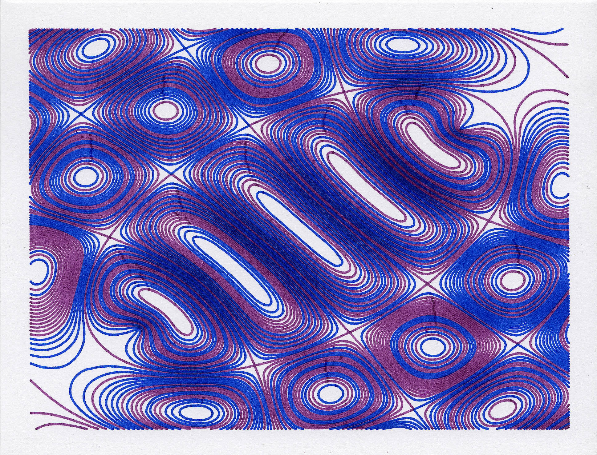
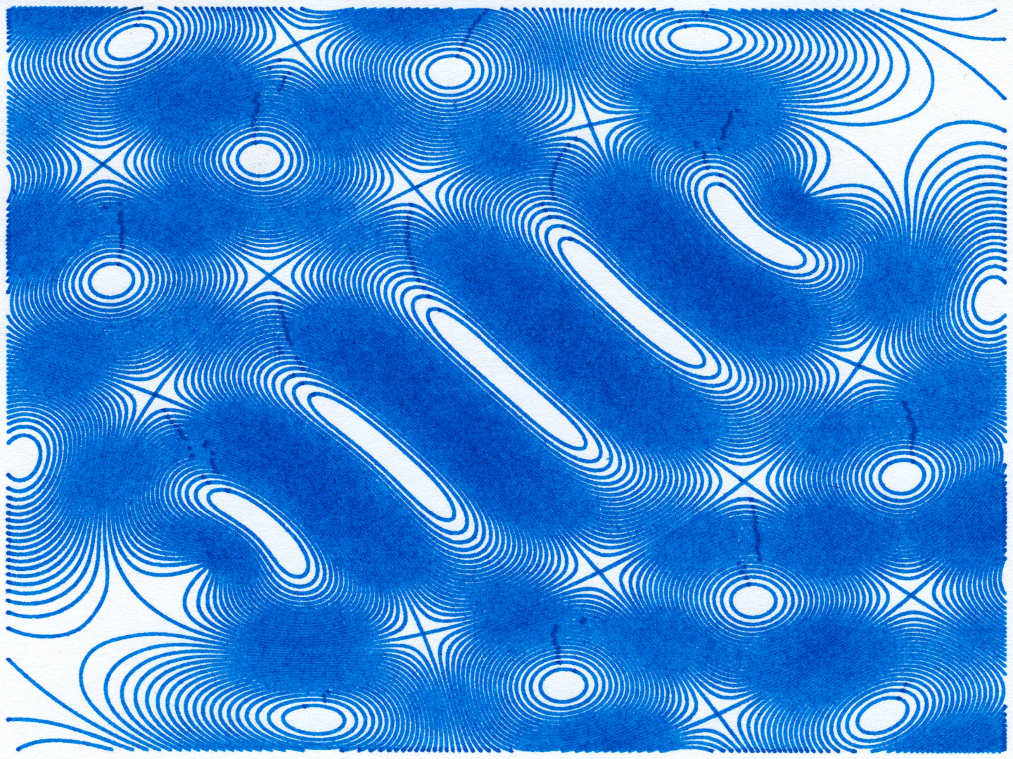
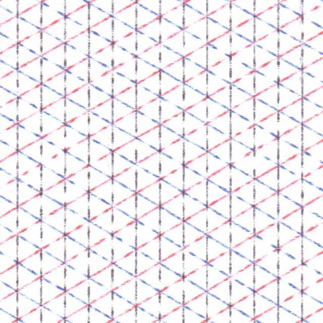
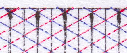
drawn using a Roland DXY-1300 plotter on Strathmore Multimedia using DeSerres medium tip pens, ~60 minutes plotting time, 180 ×180 mm
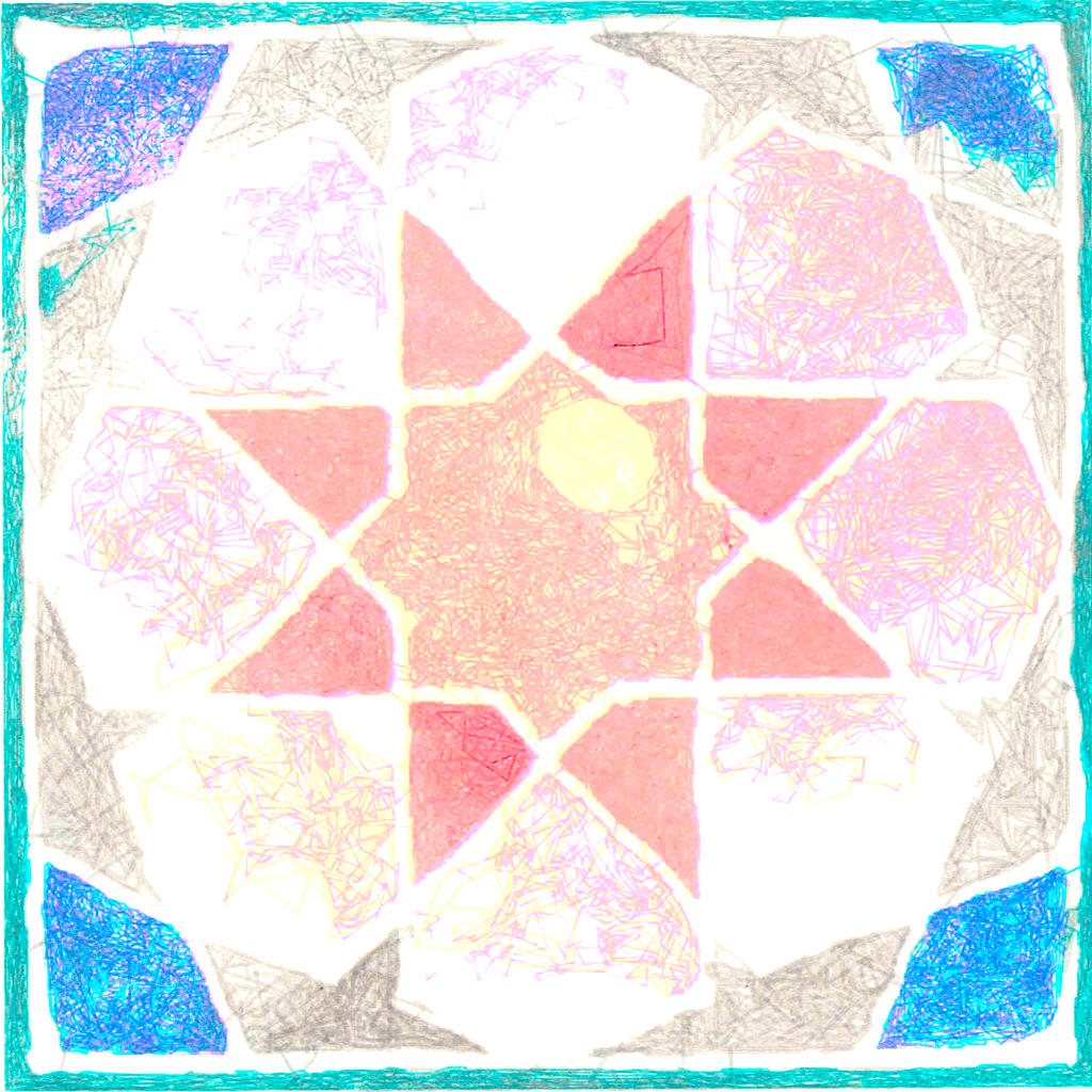
After a tonne of faffing about, I finally got something out of my plotter using Drawing Bot. I’d heard about it during the Bold Machines’ Intro to Pen Plotters course I’m taking, and the results that other people were getting looked encouraging. But for me, they weren’t great.
Maybe I was choosing too large images, but my main problem was ending up with plots with far too many lines: these would take days to plot. The controls on Drawing Bot also seemed limited: density and resolution seemed to be the only controls that do much. Drawing Bot itself wasn’t very reliable: it would sometimes go into “use all the cores!” mode when it was supposed to be idling. It would also sometimes zoom in on part of the image and fail to unzoom without quitting. Is a 32 GB i7 8-core (oldish, but still game) too little for this software? Forget any of the Voronoi plots if you want to see results today.
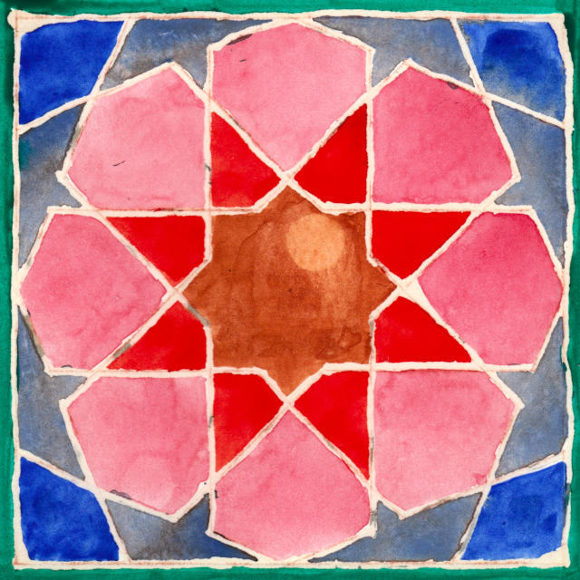
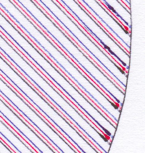
The source image was a geometric tile that I’d frisketed out years ago, forgotten about, and then found when I unstuck it from under a stack of papers. It’s somewhat artisanally coloured by me in watercolour, and the mistakes and huge water drop are all part of its charm:
source image for plotter output
If WordPress will allow an SVG, here’s what Drawing Bot made of it:
Drawing Bot SVG output: yes, it’s that faint
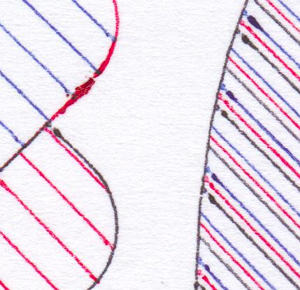
I do like the way that Drawing Bot seems to have ignored some colours, like the rose pink around the outside. The green border really is mostly cyan with a touch of black.
I haven’t magically found perfect CMYK pens in HP/Roland pen format. I couldn’t even find the Schwan-Stabilo Point 88 pens that Lauren Gardner at Bold Machines recommends. But the local DeSerres did deliver a selection of their own-brand 1.0mm Mateo Markers that are physically close to the Point 88s in size, but use a wider 1 mm fibre tip. They are also cheap; did I mention that?
The colours I chose were:
for cyan: Mint Green; RGB colour: #52C3A5; SKU: DFM-53
for magenta: Neon Pink; RGB colour: #FF26AB; SKU: DFM-F23
for yellow: Neon Yellow; RGB colour: #F3DE00; SKU: DFM-F01
for black: Green Grey 5; RGB colour: #849294; SKU: DFM-80
The RGB colours are from DeSerres’ website, and show that I’m not wildly off. Target process colours are the top row versus nominal pen colours on the bottom:
yes, there are fluo colours in there
I knew to avoid pure black, as it would overpower everything in the plot.
Overall, it plotted quite well. I plotted directly from Inkscape, one layer/pen at a time, from light (yellow) to dark (grey). Using the pen 1 slot had its disadvantages: the DXY has little pen boots to stop the pens drying, but these unfortunately get filled with old ink. The scribbly dark markings in the NNE and SSW orange kites in the plot are from the yellow pen picking up old black ink from the pen boot. Next time I’ll clean the plotter better.
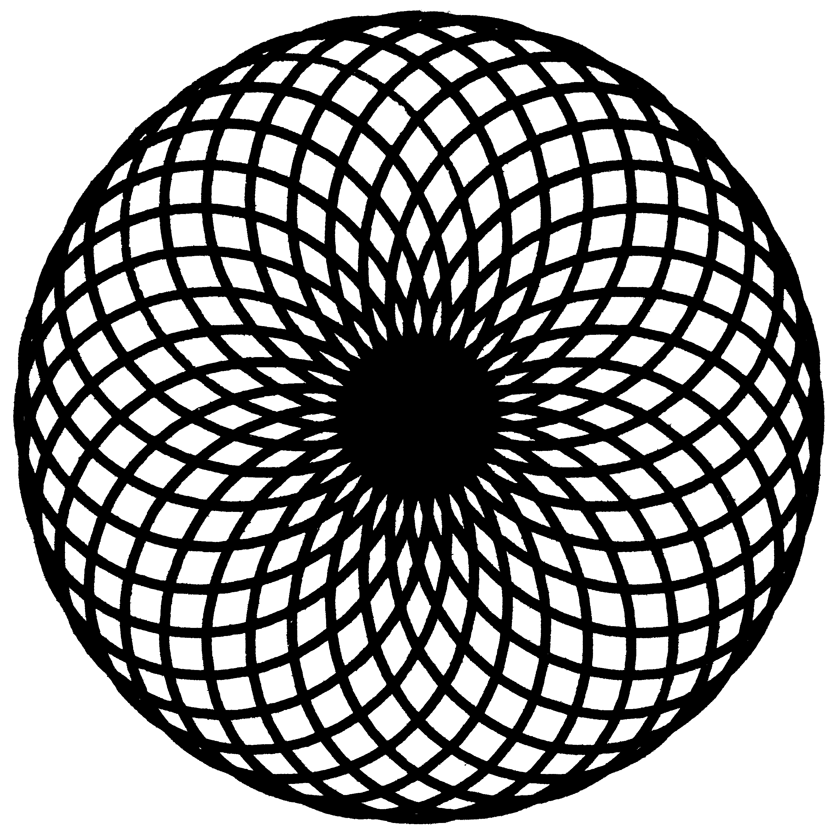
The two orbits of 16-bit RANDU, plotted as X-Y coordinates
I’d previously mentioned RANDU — IBM’s standard scientific PRNG in the 1970s that was somewhat lacking, to say the least — some time ago, but I found a new wrinkle.
For their 1130 small computer system, IBM published the Scientific Subroutine Package [PDF], which included a cut-down version of RANDU for this 16-bit machine. The code, on page 64 of the manual, doesn’t inspire confidence:
c     RANDU - from IBM Scientific Subroutine
c     Package Programmer's Manual
c     1130-CM-02X - 5th ed, June 1970
c     http://media.ibm1130.org/1130-106-ocr.pdf

      SUBROUTINE RANDU(IX, IY, YFL)
      IY = IX * 899
      IF (IY) 5, 6, 6
 5    IY = IY + 32767 + 1
 6    YFL = IY
      YFL = YFL / 32727.
      RETURN
      END
(If you’re not hip to ye olde Fortran lingo, that bizarre-looking IF statement means IF (IY < 0) GO TO 5; IF (IY == 0) GO TO 6; IF (IY > 0) GO TO 6)
It accepts an odd number < 32768 as a seed, and always outputs an odd number. Yes, it basically multiplies by 899, and changes the sign if it rolls over. Umm …
There are two possible orbits for this PRNG, each 8192 entries long:
made with gcmc and some fiddling about in Inkscape
Since I have the MidTBot ESP32 plotter running properly, I thought I should look at better ways of generating G-Code than using BASIC and lots of print statements. Ed Nisley — from whom I’ve learned a lot — always seems to be doing interesting things using the gcmc – G-Code Meta Compiler, and it looks like a useful little language to learn.
Here’s the code to make at least half of the above:
/*
   osculating circles - scruss, 2021-01
   gcmc version

   Usage with midTbot / grbl_esp32:

   gcmc osccirc.gcmc | grep -v '^G64' > osccirc.gcode

   Or for SVG:

   gcmc --svg --svg-no-movelayer --svg-toolwidth=0.25 osccirc.gcmc | sed 's/stroke:#000000/stroke:#C80022/g;' > osccirc.svg

*/
comment("osculating circles - scruss, 2021-01");

/* machine constants */
up 	      = [-, -, 5.0mm];
down 	      = [-, -, 0.0mm];
park 	      = [5.0mm, 145.0mm, 5.0mm];
feedrate(6000mm);

/* model parameters */
centre	      = [100.0mm, 75.0mm];
r	      = 65.0mm;
lim_r	      = 3.0mm;
pr	      = r;
a	      = 0.0deg;
da	      = 6.0deg;
sc	      = 0.95;
comment("centre: ", centre, "; r: ", r, "; lim_r: ", lim_r, "; pr: ", pr, "; a: ", a, "; da: ", da, "; sc: ", sc);

/* counter / sense marker */
n	      = 0;

goto(up);
do {
   centre += [(pr-r)*cos(a), (pr-r)*sin(a)];
   goto([centre.x - r, centre.y]);
   goto(down);
   n++;
   if (n%2) {
      circle_cw(centre);
   }
   else {
      circle_ccw(centre);
   }
   goto(up);
   a += 360.0deg + da;
   a %= 360.0deg;
   pr = r;
   r *= sc;
} while (r >= lim_r);

/* end */
comment(n, " circles");
goto(park);
this, but with alternate lines from the plot file drawn with alternate pens. The original was slow because it had a point roughly every 0.1 mm, and this has been smoothed. Still took maybe 15-20 minutes to draw, though.
select this to see the full resolution scan. Original is just under 6 cm wide
Unfortunately, an earlier attempt to print this figure using a fresh-out-the-box 20+-year-old HP SurePlot ¼ mm pen on glossy drafting paper resulted in holes in the paper and an irreparably gummed-up pen. If anyone knows how to unblock these pens, I’m all ears …
I made this two-colour plotted card for the MeFi “holiday card exchange – v.e.†thing. Pen plotter is a Roland DG DXY-1300 (1990s) using Roland 0.3 mm fibre-tip pens. Plot size is 123 × 91 mm, and is driven entirely from Inkscape 0.92.
Pen plotters were pretty expensive and complex pieces of electromechanical equipment. While they often earned their keep in the CAD office, they also had a function that’s almost forgotten: they could be used as input devices, too.
As a kid, we sometimes used to drive past the office of Ferranti-Cetec in Edinburgh. They specialized in digitizers: great big desk or wall mounted devices for capturing points from maps and drawings. Here’s one of their 1973 models:
While the technology and size have changed a bit, these huge bits of engineering kit are the ancestors of today’s track pads and touch screens.
Realizing that their plotters had very precise X-Y indexing and that they had two-way communications to a computer, HP made a drafting sight that fitted in place of a pen on their plotters:
HP drafting sight, part no 09872-60066.
This is a very pleasing piece of kit, all metal, thick plastic and polished optical glass. They show up on eBay occasionally, and aren’t cheap. With a bit of coercion, it fits into my HP plotter like this:
Drafting sight in HP7470A plotter
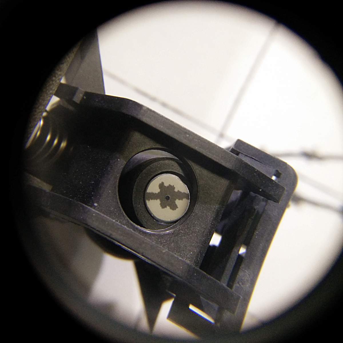
The image is very bright and clear:
Drafting sight near an axis labelDrafting sight over a point, showing cursor dot
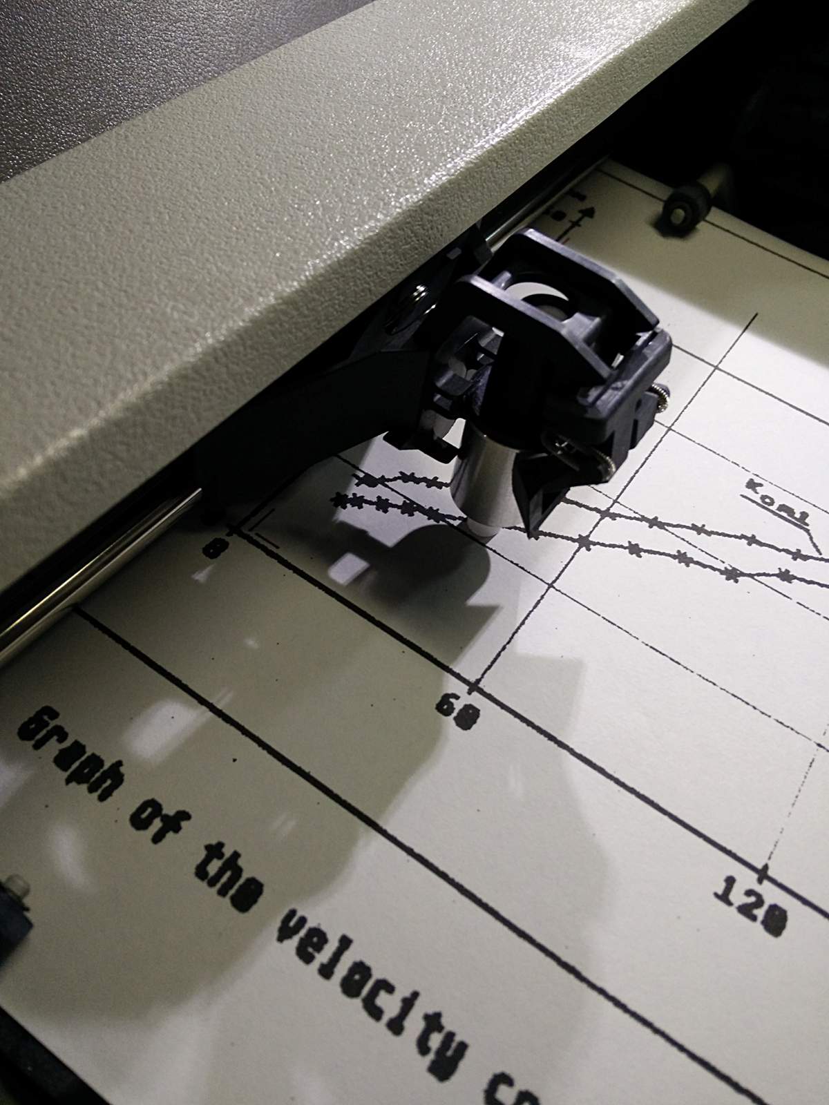
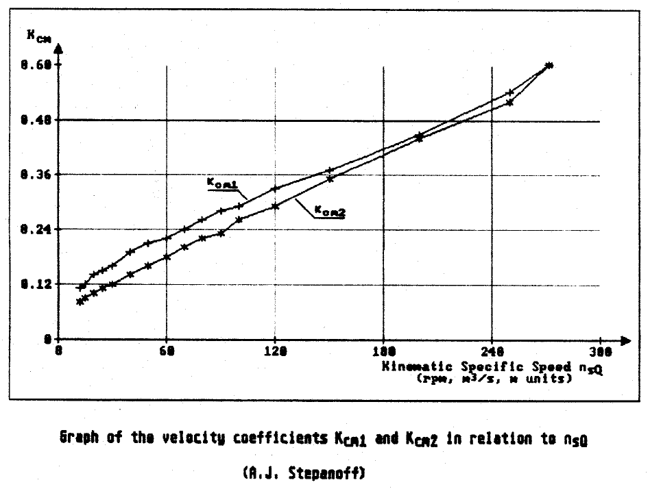
If one has a digitizing sight, one needs to find something to digitize post haste. I’m sure everyone can sense the urgency in that. So I found this, a scan from my undergraduate project writeup (centrifugal pump impeller design ftw, or something), which was probably made on an Amiga or Atari ST:
It’s a graph, with pointy bits on it
I printed this as large as I could on Letter paper, as it’s the only size my HP7470A plotter can take. Now all it needed was a small matter of programming to get the data from the plotter. Here’s a minimally-useful digitizer for HP and compatible serial plotters. Although I ran it on my little HP grit wheel plotter attached to a Raspberry Pi, I developed it with my larger Roland plotter. The only fancy module it needs is pySerial.
#!/usr/bin/env python
# -*- coding: utf-8 -*-
# a really crap HP-GL point digitizer
#  scruss - 2016

from time import sleep
from string import strip
import serial

ser = serial.Serial(port='/dev/ttyUSB1', baudrate=9600, timeout=0.5)
lbl = ''
points = []
labels = []
k = 0
retval = 0

ser.write('DP;')                # put in digitizing mode
while lbl != 'quit':
    ser.write('OS;')
    ret = strip(ser.read(size=5), chr(13))
    print ('Retval: ', ret)
    if ret != '':
        retval = int(ret)
    if retval & 4:              # bit 2 is set; we have a point!
        print ('Have Point! Retval: ', retval)
        retval = 0
        ser.write('OD;')
        pt = strip(ser.read(size=20), chr(13))
        print ('OD point: ', pt)
        lbl = raw_input('Input label [quit to end]: ')
        points.append(pt)
        labels.append(lbl)
        k = k + 1
        ser.write('DP;')        # put in digitizing mode again
    sleep(1)
ser.close()

f = open('digit.dat', 'w')
for i in range(k):
    f.write(points[i])
    f.write(',')
    f.write(labels[i])
    f.write('\n')
f.close()
In the unlikely event that anyone actually uses this, they’ll need to change the serial port details near the top of the program.
The program works like this:
Move the drafting sight to the point you want to capture using the plotter’s cursor keys, and hit the plotter’s ENTER key
Your computer will prompt you for a label. This can be anything exceptquit, that ends the program
When you have digitized all the points you want and entered quit as the last label, the program writes the points to the file digit.dat
I didn’t implement any flow control or other buffer management, so it can crash in a variety of hilarious ways. I did manage to get it to work on the lower trace of that graph, and got these data:
The first two columns are X and Y, in HP-GL units — that’s 1/40 mm, or 1/1016 inches. The third column will always be 1 if you have the sight down. The last columns are the label; if you put commas in them, opening the file as CSV will split the label into columns. I used it to fudge axis points. You’ll also note that the last three lines of data are my valiant attempts to quit the program.
Assuming the axes are not skewed (they are, very slightly, but shhh) some simple linear interpolation gives you the results below:
(For prettier things to do with plotter digitizing commands, Ed Nisley KE4ZNU has made some rather lovely Superformula patterns)
If you don’t have a plotter, or even if you do and you don’t have hours to waste mucking about with Python, obsolete optics and serial connections, Ankit Rohatgi’s excellent WebPlotDigitizer (or Engauge, as I found out when this article hit HackerNews in 2021) gets numbers out of graphs quickly. It handles all sorts of graphs rather well.
Update, 2025: eek, but WebPlotDigitizer is now login-only and has been infested by AI shite. Run away now, run away fast … or try to find an old mirror online, such as WebPlotDigitizer at utk.edu.
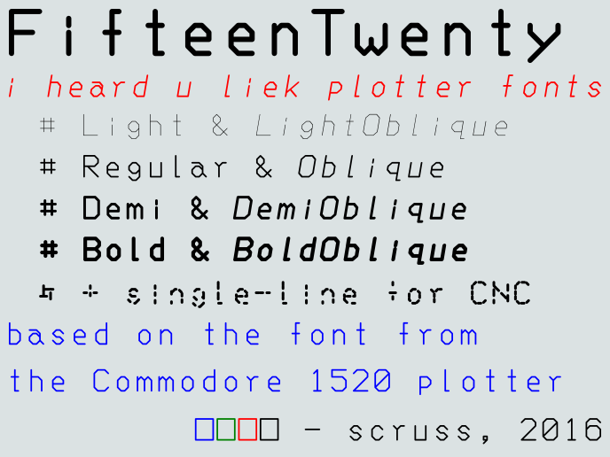
Update, September 2016: this font was officially squee‘d over by Josh “cortex” Millard on the Metafilter Podcast #120: Hard Out There For A Nerd. I had the great pleasure of meeting Josh at XOXO 2016, too.
The Commodore 1520 was a tiny pen plotter sold for the Commodore 64 home computer. It looked like this:
I never owned one, but it seems it was more of a curiosity than a useful product.
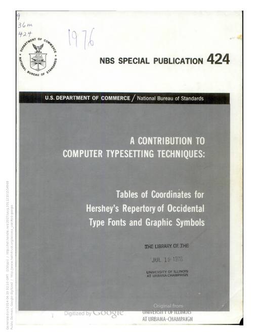
From a nerdy point of view, however, this device was rather clever in that it packed a whole plotter command language, including a usable font, into 2048 bytes of ROM. Nothing is that small any more.
Based on my work with the Hershey font collection, I thought it would be fun to extract the coordinates and make a real OpenType font from these data. I’m sure others would sense the urgency in this task, too.
Since Commodore computers used a subset of ASCII, there’s a barely-usable set of characters in this first release. Notable missing characters include:
U+005C    \    REVERSE SOLIDUS
U+005E    ^    CIRCUMFLEX ACCENT
U+0060    `    GRAVE ACCENT
U+007B    {    LEFT CURLY BRACKET
U+007C    |    VERTICAL LINE
U+007D    }    RIGHT CURLY BRACKET
U+007E    ~    TILDE
I’ll get to those later, perhaps.
Huge thanks to all who helped get the data, and make the bits of software I used to make this outline font.
(Note: although the Project 64 Reloaded contains some extraction code to nominally produce an SVG font, it doesn’t work properly — and SVG fonts are pretty much dead anyway. I didn’t base any of my work on their Ruby code.)
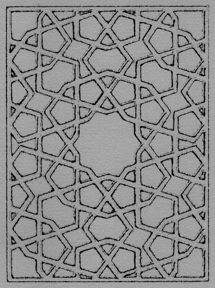
Well, I didn’t expect that to happen. I was plotting this simple girih frame when something went wrong, and the plotter slammed the (new-old stock, almost unused … sniff) HP drafting pen into the side of the thick watercolour paper, breaking off the tip.
I didn’t notice the damage, so I restarted the plot, and the above smeary and uncertain lines came out. It’s certainly more organic than a mechanical plot would tend to be …
After a relative lack of success in making cheap plotter pens, I managed to score a trove of old pens on eBay. Some of these were dry, and I tried to resuscitate them. A few came back to life, but I ended up with a handful of very dead pen shells.
A dry plotter pen, possibly Alvin
I think the pens were made or sold by Alvin, as there were several empty Alvin trays in the batch I got on eBay. In taking one apart, I thought that a pen refill might just slide inside. Lo and behold, but didn’t the pen nerd’s fave gel pen du jour refill just slide in with enough of an interference fit that it wouldn’t easily slide back out.
Taking the dry pens apart isn’t too easy:
Pull the black tip straight out with pliers; it has a long fibre plug which goes into the ink reservoir. Discard the tip.
While it’s really hard to see, the other end of the pen body has a push-on plug. Gently working around it with a sharp knife can open it up a bit.
Once you’re inside the pen, pull the dry fibre ink reservoir out with tweezers and discard it.
Converting the pen body to use a Jetstream refill needs some tools:
Drill a hole in the plug at the end of the pen body just large enough to allow the end of the refill to pass through. It helps if this is mostly centred to keep the pen point centred; this is important for accurate plots.
Cut a piece of tubing just wide enough to slip over the pen refill, but not quite narrow enough to fit through the hole you just drilled. I used some unshrunk heatshrink tubing for this. It needs to be just long enough to push against the plug when the pen tip is at the right length. This should help stop the refill getting hammered back into the body by your plotter.
Before you assemble the pen, I find it useful to cut a couple of flats in the sides of the plug so you can more easily change the refill. You don’t have to do this, though.
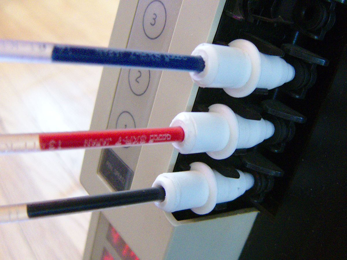
Assemble the pen:
Push the Jetstream refill into the pen body, and adjust it so it sticks out about 6 mm clear of the plastic collar near the nib.
Put the tubing over the other end of the refill, and push the plug over the top, clicking it into place.
Three pens in place on my DXY-1300
To get best results, you’ll have to slow your plot speed down quite a bit. At standard speeds, you get a ¼ mm interrupted line which looks like this:
Jetstream at full speed
Close up, the lines are really faint
A hint that I should run them slower was at the start of each line, where the line would start very thick, then taper off as the ink supply ran low:
acceleration blobs
Run at 120 mm/s, the results where a bit darker, but still blobby at the start of lines:
120 mm/s
Slowing down to 60 mm/s produced slightly better results:
60 mm/s
But sharpest of all was at the crawling speed 30 mm/s:
30 mm/s
Some pronounced blobs at the starts of lines still. Here’s the full page at 600 dpi, squished into a very lossy PDF: jetstream_plotter-slow
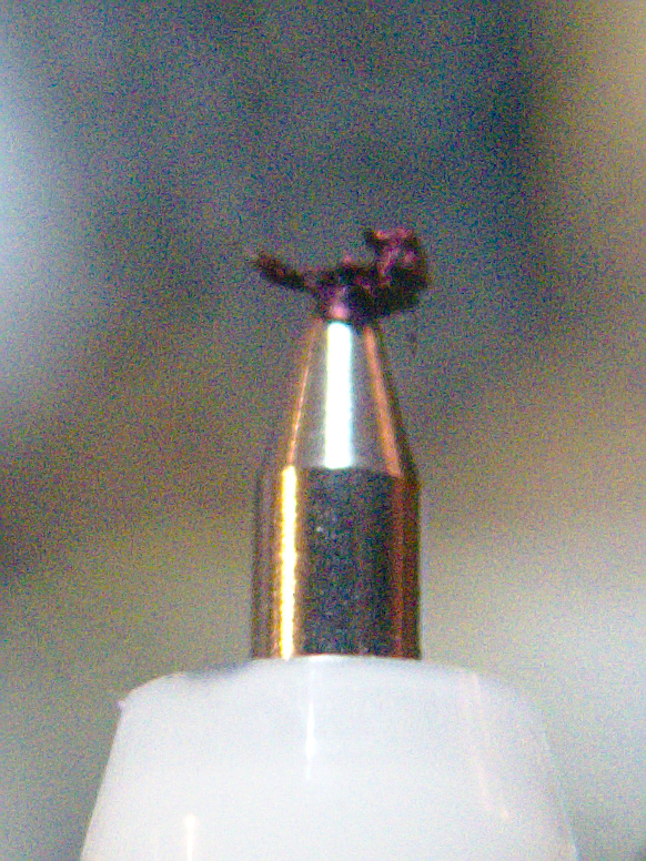
The blobs could be due to this, though:
grode on pen tip
It seems that a mix of paper fibres and coagulated ink builds up on the tip. Occasional cleaning seems to be a good idea. It also seems to help to draw a quick scratch line before anything important so the ink will be flowing properly.
Just to sign off, here’s one of the pens in action:
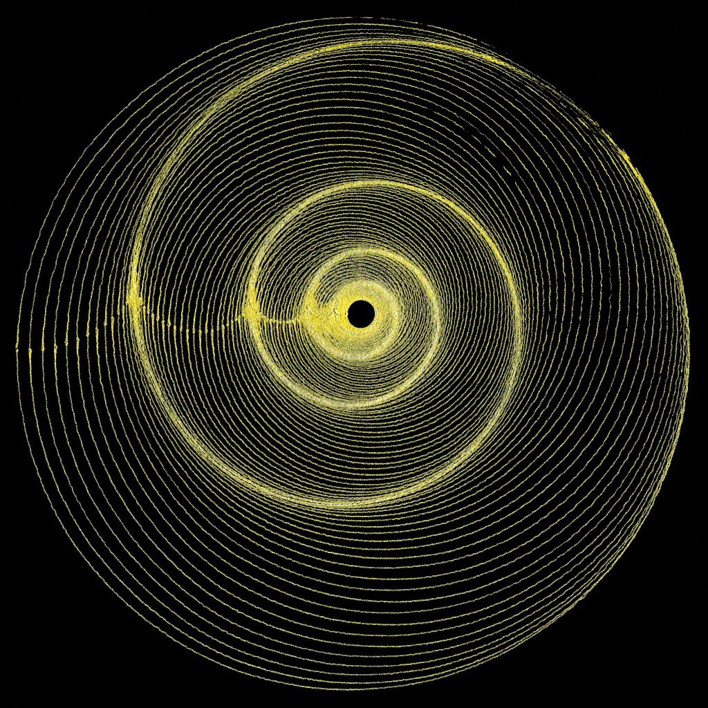
Inspired by Robert Howsare’s Drawing Apparatus, a time-step simulation of a similar apparatus was developed. Each trace was made of thousands of straight line segments, one for each rotation of the turntables’ drive motors, and enough to create a closed figure. Suitable gearing was modelled to simulate standard (North American) gramophone speeds of 16⅔, 33⅓, 45 and 78⅕ rpm for each of the turntables. Drive crank lengths were derived from standard record sizes. The initial starting angle of each turntable was also modelled.
Three simulation runs were chosen and superimposed. The result was plotted on “A” size vellum using 0.3 mm ceramic drafting pens. Total plot time at 90 mm/s: 22 minutes.
Code available on request.
(update, 2026: Code available on request if I can find it. I have implemented this project from scratch at least three different times because I forgot I’d done it before. You might say I’m forgetful, but I say I get 3× the joy of discovery this way …)
![[decorative] a spiralling figure made of scaled and rotated equilateral triangles](https://scruss.com/wordpress/wp-content/uploads/2025/04/hpgl-rotatey.png)
![[decorative] a spiralling figure made of scaled and rotated equilateral triangles](https://scruss.com/wordpress/wp-content/uploads/2025/04/20250408_214147_BRWD89C6730425A_000572a-787x1024.jpg)


.jpg#/media/File:Commodore_1520_printer_plotter_(adjusted).jpg)


