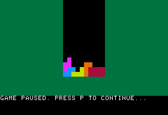
cp2up.sh — fits the important part of Canada Post print labels two per sheet

blurred (for privacy) 2-up landscape page of Canada Post Tracked Package (to USA) shipping labels made by this script
no you will not read my 2-up shipping labels

If you need to ship things, you’re probably not too keen on queuing at the post office right now. Canada Post’s Ship Online service is pretty handy if you have a printer. The PDFs it produces are okay to print on plain paper, but if you’re using full-sheet labels like Avery 5165 you’re going to waste half a sheet of expensive labels.

If you’ve got two parcels to mail, this shell script will extract the right side of each page and create a single 2-up PDF with both your labels on the same page. You will need:

On my Ubuntu system, you can get good-enough¹ versions by doing this:

sudo apt install poppler-utils netpbm img2pdf

The code:

#!/bin/bash
# cp2up.sh - fits the important part of Canada Post print labels 2 per sheet
# scruss, 2021-05 - CC-BY-SA
# hard-coded input name (document.pdf)
# hard-coded output name (labels-2up.pdf)
# accepts exactly two labels (sorry)

dpi=600
width_in=11
height_in=8.5
# png intermediate format uses pixels per metre
dpm=$(echo "scale=3; $dpi * 1000 / 25.4" | bc)
# calculated pixel sizes, truncated to integer
half_width_px=$(echo "$width_in * $dpi / 2" | bc | sed 's/\..*$//')
height_px=$(echo "$height_in * $dpi" | bc | sed 's/\..*$//')

pdftoppm -mono -r "$dpi" -x "$half_width_px" -y 0 \
	 -W  "$half_width_px" -H "$height_px" document.pdf labels
pnmcat -lr labels-1.pbm labels-2.pbm |\
    pnmtopng -compression 9 -phys "$dpm" "$dpm" 1 > labels.png \
    && rm labels-1.pbm labels-2.pbm
# fix PDF time stamps
now=$(date --utc --iso-8601=seconds)
img2pdf -o labels-2up.pdf --creationdate "$now" --moddate "$now" \
	--pagesize "Letter^T" labels.png \
    && rm labels.png 

# saved from:
# history | tail | awk '{$1=""; print}' |\ 
#           perl -pwle 'chomp;s/^\s+//;' > cp2up.sh

It’s got a few hard-coded assumptions:

  • input name (document.pdf);
  • output name (labels-2up.pdf);
  • accepts exactly two labels (sorry).

Clever people could write code to work around these. Really clever people could modify this to feed a dedicated label printer.

Yes, I could probably have done all this with one ImageMagick command. When ImageMagick’s command line syntax begins to make sense, however, it’s probably time to retire to that remote mountain cabin and write that million-word thesis on a manual typewriter. Also, ImageMagick’s PDF generation is best described as pish.

One of the issues that this script avoids is aliasing in the bar-codes. For reasons known only to the anonymous PDF rendering library used by Canada Post, their shipping bar-codes are stored as smallish (780 × 54 px) bitmaps that are scaled up to a 59 × 19 mm print size. Most PDF viewers (and Adobe Viewer is one of these) will anti-alias scaled images, making them slightly soft. If you’re really unlucky, your printer driver will output these as fuzzy lines that no bar-code scanner could ever read. Rendering them to high resolution mono images may still render the edges a little roughly, but they’ll be crisply rough, and scanners don’t seem to mind that.

split image of simulated printed barcode: top image is five indistinct black-grey bars merging into a white background, bottom image is the same vertical lines, rendered crisply but showing some slightly rough edges
fuzzy vs crisply rough: scaled image (top) vs direct-rendered (bottom), at simulated 600 dpi laser print resolution

¹: Debian/Ubuntu’s netpbm package is roughly 20 years out of date for reasons that only a very few nerds care about, and the much better package is blocked by Debian’s baroque and gatekeepery packaging protocol. I usually build it from source for those times I need the new features.

Endless screaming in URL

A friend introduced me to A(x56) – URL Lengthener — perhaps better known as https://aaa.aaaaaaaaaaaaaaaaaaaaaaaaaaaaaaaaaaaaaaaaaaaaaaaaaaaaaaaa.com/. Consequently, this website should in future be referred to as https://aaa.aaaaaaaaaaaaaaaaaaaaaaaaaaaaaaaaaaaaaaaaaaaaaaaaaaaaaaaa.com/a?áaaÂáaaÂáaaÂáaaÂáaaÂáaaÂáaaÂáaaÂáaaÂáaaÂáaaÂáaaÂáaaÂáaaÂáaaÂáaaÂáaaÂáaaÂáaaÂáaaÂáaaÂáaaÂáaaÂáaaÂáaaÂáaaÂáaaÂáaaÂáaaÂáaaÂáaaÂáaaÂáaaÂáaaÂáaaÂáaaÂáaaÂáaaÂåAæãæãæaæââÁáÆáÆæâåâæáæäæâæâáÅåâåÆåÄáÆåáåÃåÆåæáÆ.

It sounds even better than it reads:

that URL, as read by Flite

Applied Futility: Re-creating RAND’s ‘A Million Random Digits’

Sometimes, one must obey the inscrutable exhortations of one’s soul and travel deep into the inexplicable. The planet Why? has been left far behind, the chatter of its querulous denizens nothing more than a faint wisp of static. Where I’m going, pure patternlessness is all there is.

Page 53 from “A Million Random Digits …”, showing the five-digit sequential line number at left, followed by ten columns of five random digits each
A page from “A Million Random Digits …”, showing the five-digit sequential line number at left, followed by ten columns of five random digits each

In 1955, military-industrial complex stalwarts RAND Corporation published a huge book of just pages and pages of … digits. The digits were deliberately as random as possible, and were intended to help the fledgling practice of data science carry out truly random simulations. The book was called “A Million Random Digits with 100,000 Normal Deviates”. It was also made available on punched cards, with 50 digits to a card adding up to ten boxes of 2000 cards. A single box of punched cards was about 370 × 200 × 95 mm and weighed roughly 5 kg, so these digits had heft.

I thought it might be fun (or perhaps fun?: pronounced with a rising, questioning tone to stress the might-ness of any enjoyment arising) to dig into how RAND carried out this work, create some electronics to produce a similar random stream, and see how my random digits compare for randomness with RAND’s. For a final trick, I might even typeset the whole giant table into a book that no-one wants.

As I research and progress with this project, I’ll add in links here

I must stress: there is no reason for me to do this. A $5 micro-controller board can generate tens to hundreds of thousands of truly random digits per second. Any results I produce will have no use beyond my own amusement.


A Million Random Digits with 100,000 Normal Deviates is © Copyright 2001 RAND. Apart from a couple of page images and quotations from supporting material, none of that work is reproduced here. RAND does not support or endorse my futile efforts in any way.

Delicate tracings from a terrible PRNG

The two orbits of 16-bit RANDU, plotted as X-Y coordinates

I’d previously mentioned RANDU — IBM’s standard scientific PRNG in the 1970s that was somewhat lacking, to say the least —some time ago, but I found a new wrinkle.

For their 1130 small computer system, IBM published the Scientific Subroutine Package [PDF], which included a cut-down version of RANDU for this 16-bit machine. The code, on page 64 of the manual, doesn’t inspire confidence:

c     RANDU - from IBM Scientific Subroutine 
c     Package Programmer's Manual
c     1130-CM-02X - 5th ed, June 1970
c     http://media.ibm1130.org/1130-106-ocr.pdf

      SUBROUTINE RANDU(IX, IY, YFL)
      IY = IX * 899
      IF (IY) 5, 6, 6
 5    IY = IY + 32767 + 1
 6    YFL = IY
      YFL = YFL / 32727.
      RETURN
      END

(If you’re not hip to ye olde Fortran lingo, that bizarre-looking IF statement means IF (IY < 0) GO TO 5; IF (IY == 0) GO TO 6; IF (IY > 0) GO TO 6)

It accepts an odd number < 32768 as a seed, and always outputs an odd number. Yes, it basically multiplies by 899, and changes the sign if it rolls over. Umm …

There are two possible orbits for this PRNG, each 8192 entries long:

  1. Starting seed 1 (899, 21769, 7835, …, 18745, 9003, 1, 899)
  2. Starting seed 5 (4495, 10541, 6407, …, 28189, 12247, 5, 4495).

The plot above is the first series as X and the second as Y. I used INTEGER*2 types to simulate the 1130’s narrow integers.

Niche Knowledge: Z80 parallel port SD card on Zeta2

green circuit board with secure digital card slot on left and 40-pin parallel interface connectors on the right
Mini PPISD board: a slow SD card mass-storage system for 8-bit computers

Almost no-one will need this knowledge, but I might need to remember it. In order to add Mini PPISD support to a RomWBW 3.01-supported system, you need to create a file called something like Source/HBIOS/Config/ZETA2_ppisd.asm (for yes, I’m using a Zeta SBC V2) containing:

#include "cfg_zeta2.asm"
UARTCFG		.SET	UARTCFG | SER_RTS
CRTACT		.SET	TRUE		
PPIDEENABLE	.SET	FALSE		
SDENABLE	.SET	TRUE		
PPPENABLE	.SET	FALSE		
PPISD		.EQU	TRUE

Running make from the top-level directory should create a ROM image called Binary/ZETA2_ppisd.rom for you to write to flash. Since my floppy drive isn’t feeling too happy, I had to resort to buying a TL866II Plus programmer to write the chip.

And it worked!

 RomWBW HBIOS v3.0.1, 2021-03-12

 ZETA V2 Z80 @ 8.000MHz
 0 MEM W/S, 1 I/O W/S, INT MODE 2
 512KB ROM, 512KB RAM

 CTC: MODE=Z2 IO=0x20
 UART0: IO=0x68 16550A MODE=38400,8,N,1
 DSRTC: MODE=STD IO=0x70 Sun 2021-03-14 17:47:13 CHARGE=OFF
 MD: UNITS=2 ROMDISK=384KB RAMDISK=384KB
 FD: IO=0x30 UNITS=2
 SD: MODE=PPI IO=0x60 DEVICES=1
 SD0: SDSC NAME=SD    BLOCKS=0x003C7800 SIZE=1935MB

 Unit        Device      Type              Capacity/Mode
 ----------  ----------  ----------------  --------------------
 Char 0      UART0:      RS-232            38400,8,N,1
 Disk 0      MD1:        RAM Disk          384KB,LBA
 Disk 1      MD0:        ROM Disk          384KB,LBA
 Disk 2      FD0:        Floppy Disk       3.5",DS/HD,CHS
 Disk 3      FD1:        Floppy Disk       3.5",DS/HD,CHS
 Disk 4      SD0:        SD Card           1935MB,LBA

 ZETA V2 Boot Loader

 ROM: (M)onitor (C)P/M (Z)-System (F)orth (B)ASIC (T)-BASIC (P)LAY (U)SER ROM  
 Disk: (0)MD1 (1)MD0 (2)FD0 (3)FD1 (4)SD0 

 Boot Selection? 

I was pleasantly surprised how easy it is to use a TL866 programmer under Linux. minipro does all the work, though. To write and verify the whole 512K Flash ROM, it’s:

minipro -p SST39SF040 -w ZETA2_ppisd.rom

The programmer supports over 16000 devices, of which around 10000 are variants (form factor, programming voltage, speed, OTP, etc). It’ll also verify over 100 different 74-series logic chips. It’s not a super cheap device (mine was a little over $80, from Simcoe Diy) but it does a lot for that price.

Next stop: try rebuilding BBC BASIC with RomWBW’s timer support included ..

Seeeduino XIAO simple USB volume control with CircuitPython

round computer device with USB cable exiting at left. Small microcontroller at centreshowing wiring to LED ring and rotary encoder
Slightly blurry image of the underside of the device, showing the Seeeduino XIAO and the glow from the NeoPixel ring. And yes, the XIAO is really that small

Tod Kurt’s QTPy-knob: Simple USB knob w/ CircuitPython is a fairly simple USB input project that relies on the pin spacing of an Adafruit QT Py development board being the same as that on a Bourns Rotary Encoder. If you want to get fancy (and who wouldn’t?) you can add a NeoPixel Ring to get an RGB glow.

The QT Py is based on the Seeeduino XIAO, which is a slightly simpler device than the Adafruit derivative. It still runs CircuitPython, though, and is about the least expensive way of doing so. The XIAO is drop-in replacement for the Qt Py in this project, and it works really well! Everything you need for the project is described here: todbot/qtpy-knob: QT Py Media Knob using rotary encoder & neopixel ring

I found a couple of tiny glitches in the 3d printed parts, though:

  1. The diffuser ring for the LED ring is too thick for the encoder lock nut to fasten. It’s 2 mm thick, and there’s exactly 2 mm of thread left on the encoder.
  2. The D-shaft cutout in the top is too deep to allow the encoder shaft switch to trigger.

I bodged these by putting an indent in the middle of the diffuser, and filling the top D-shaft cutout with just enough Blu Tack.

Tod’s got a bunch of other projects for the Qt Py that I’m sure would work well with the XIAO: QT Py Tricks. And yes, there’s an “Output Farty Noises to DAC” one that, regrettably, does just that.

Maybe I’ll add some mass to the dial to make it scroll more smoothly like those buttery shuttle dials from old video editing consoles. The base could use a bit more weight to stop it skiting about the desk, so maybe I’ll use Vik’s trick of embedding BB gun shot into hot glue. For now, I’ve put some rubber feet on it, and it mostly stays put.


Hey! Unlike my last Seeed Studio device post, I paid for all the bits mentioned here.

Nyan Cat, except it gets faster — RTTTL on the Raspberry Pi Pico

Raspberry Pi Pico with small piezo speaker connected to pins 23 (ground) and 26 (GPIO 20)
piezo between pins 26 and 23. Sounds a little like this

It was inevitable:

  1. A Raspberry Pi Pico; plus
  2. a tiny piezo PC beeper; plus
  3. MicroPython; plus
  4. dhylands / upy-rtttl; plus
  5. nyancat.rtttl; plus
  6. my unfailing sense of knowing when to stop, then ignoring it

brings you this wonderful creation, which plays the Nyan Cat theme forever, except it gets 20% faster each time. This is weapons-grade annoying (thank’ee kindly), so I’m not going to include a recording here. If you must hear an approximation, paste the RTTTL into Play RTTTL Online and enjoy.

# Raspberry Pi Pico RTTTL example
# nyan cat, but it gets faster
# scruss - 2021-02: sorry, not sorry ...

# Uses rtttl.py from
#  github.com/dhylands/upy-rtttl
# Nyan Cat RTTTL from
#  github.com/KohaSuomi/emb-rtttl/blob/master/rtttl/nyancat.rtttl

from rtttl import RTTTL
from time import sleep_ms
from machine import Pin, PWM

b = 90    # bpm variable

# pin 26 - GP20; just the right distance from GND at pin 23
#  to use one of those PC beepers with the 4-pin headers
pwm = PWM(Pin(20))
led = Pin('LED', Pin.OUT)


def play_tone(freq, msec):
    # play RTTL notes, also flash onboard LED
    print('freq = {:6.1f} msec = {:6.1f}'.format(freq, msec))
    if freq > 0:
        pwm.freq(int(freq))       # Set frequency
        pwm.duty_u16(32767)       # 50% duty cycle
    led.on()
    sleep_ms(int(0.9 * msec))     # Play for a number of msec
    pwm.duty_u16(0)               # Stop playing for gap between notes
    led.off()
    sleep_ms(int(0.1 * msec))     # Pause for a number of msec


while True:
    nyan = 'nyancat:d=4,o=5,b=' + str(b) + ':16d#6,16e6,8f#6,8b6,16d#6,16e6,16f#6,16b6,16c#7,16d#7,16c#7,16a#6,8b6,8f#6,16d#6,16e6,8f#6,8b6,16c#7,16a#6,16b6,16c#7,16e7,16d#7,16e7,16c#7,8f#6,8g#6,16d#6,16d#6,16p,16b,16d6,16c#6,16b,16p,8b,8c#6,8d6,16d6,16c#6,16b,16c#6,16d#6,16f#6,16g#6,16d#6,16f#6,16c#6,16d#6,16b,16c#6,16b,8d#6,8f#6,16g#6,16d#6,16f#6,16c#6,16d#6,16b,16d6,16d#6,16d6,16c#6,16b,16c#6,8d6,16b,16c#6,16d#6,16f#6,16c#6,16d#6,16c#6,16b,8c#6,8b,8c#6,8f#6,8g#6,16d#6,16d#6,16p,16b,16d6,16c#6,16b,16p,8b,8c#6,8d6,16d6,16c#6,16b,16c#6,16d#6,16f#6,16g#6,16d#6,16f#6,16c#6,16d#6,16b,16c#6,16b,8d#6,8f#6,16g#6,16d#6,16f#6,16c#6,16d#6,16b,16d6,16d#6,16d6,16c#6,16b,16c#6,8d6,16b,16c#6,16d#6,16f#6,16c#6,16d#6,16c#6,16b,8c#6,8b,8c#6,8b,16f#,16g#,8b,16f#,16g#,16b,16c#6,16d#6,16b,16e6,16d#6,16e6,16f#6,8b,8b,16f#,16g#,16b,16f#,16e6,16d#6,16c#6,16b,16f#,16d#,16e,16f#,8b,16f#,16g#,8b,16f#,16g#,16b,16b,16c#6,16d#6,16b,16f#,16g#,16f#,8b,16b,16a#,16b,16f#,16g#,16b,16e6,16d#6,16e6,16f#6,8b,8a#,8b,16f#,16g#,8b,16f#,16g#,16b,16c#6,16d#6,16b,16e6,16d#6,16e6,16f#6,8b,8b,16f#,16g#,16b,16f#,16e6,16d#6,16c#6,16b,16f#,16d#,16e,16f#,8b,16f#,16g#,8b,16f#,16g#,16b,16b,16c#6,16d#6,16b,16f#,16g#,16f#,8b,16b,16a#,16b,16f#,16g#,16b,16e6,16d#6,16e6,16f#6,8b,8c#6'
    tune = RTTTL(nyan)
    print('bpm: ', b)
    for freq, msec in tune.notes():
        play_tone(freq, msec)
    b = int(b * 1.2)

Visualizing PWM

my desk is not usually this tidy

I built a DS0150 — successfully, on my second try — and wanted to measure something. My demo MicroPython program from MicroPython on the terrible old ESP8266-12 Development Board has been running since May 2020, and the RGB LED’s red channel is conveniently broken out to a header. Since the DSO150 has precisely one channel, it let me see the how the PWM duty cycle affects the voltage (and brightness) of the LED.

I can’t think of oscilloscopes without being reminded of a scene from one of my favourite sci-fi books, The Reproductive System by John Sladek. Cal, the hapless new hire in the Wompler toy factory-turned-military research lab, is showing the boss some equipment while making up more and more extravagant names for them for the clueless owner:

At each exhibit, Grandison [Wompler] would pause while Cal named the piece of equipment. Then he would repeat the name softly, with a kind of wonder, nod sagely, and move on. Cal was strongly reminded of the way some people look at modern art exhibitions, where the labels become more important to them than the objects. He found himself making up elaborate names.
“And this, you’ll note, is the Mondriaan Modular Mnemonicon.”
“—onicon, yes.”
“And the Empyrean diffractosphere.”
“—sphere. Mn. I see.”
Nothing surprised Grandison, for he was looking at nothing. Cal became wilder. Pointing to Hita’s desk, he said, “The chiarascuro thermocouple.”
“Couple? Looks like only one, to me. Interesting, though.”
A briar pipe became a “zygotic pipette,” the glass ashtray a “Piltdown retort,” and the lamp a “phase-conditioned Aeolian.” Paperclips became “nuances.”
“Nuances, I see. Very fine. What’s that thing, now?”
He pointed to an oscilloscope. Cal took a deep breath.
“Its full name,” he said, “is the Praetorian eschatalogical morphomorphic tangram, Endymion-type, but we usually just call it a ramification.”
The old man fixed him with a stern black eye. “Are you trying to be funny or something? I mean, I may not be a smart-aleck scientist, but I sure as hell know a television when I see one.”
Cal assured him it was not a television, and proved it by switching it on. “See,” he said, pointing to a pattern of square waves, “there are the little anapests.”

— The Reproductive system, by John Sladek (text copypasta from Grey Goo in the 1960s)

So we were displaying roughly 500 anapests/s there. Not bad, not bad at all …

Raspberry Pi Pico: DS18x20 in MicroPython

Updated: Thanks to Ben, who noticed the Fritzing diagrams had the sensors the wrong way round. Fixed now…

Hidden away in the Pico MicroPython guide is a hint that there may be more modules installed in the system than they let on. In the section about picotool, the guide has a seemingly innocuous couple of lines:

frozen modules: _boot, rp2, ds18x20, onewire, uasyncio, uasyncio/core, uasyncio/event, uasyncio/funcs, uasyncio/lock, uasyncio/stream

The third and fourth ‘frozen modules’ are a giveaway: it shows that support for the popular Dallas/Maxim DS18x20 1-Wire temperature sensors is built in. Nowhere else in the guide are they mentioned. I guess someone needs to write them up.

DS18x20 digital temperature sensors – usually sold as DS18B20 by Maxim and the many clone/knock-off suppliers – are handy. They can report temperatures from -55 to 125 °C, although not every sensor will withstand that range. They come in a variety of packages, including immersible sealed units. They give a reliable result, free from ADC noise. They’re fairly cheap, the wiring’s absurdly simple, and you can chain long strings of them together from the same input pin and they’ll all work. What they aren’t, though, is fast: 1-Wire is a slow serial protocol that takes a while to query all of its attached devices and ferry the results back to the controller. But when we’re talking about environmental temperature, querying more often than a few times a minute is unnecessary.

So this is the most complex way you can wire up a DS18x20 sensor:

breadboard with raspberry Pi Pico, DS18x20 sensor with 47 k? pull-up resistor between 3V3 power and sensor data line
Raspberry Pi Pico connected to a single DS18x20 sensor

and this is how it’s wired:

   DS18X20    Pico
   =========  =========
   VDD      ? 3V3
              /
     --47 k?--
    /
   DQ       ? GP22
   GND      ? GND

 (47 k? resistor between DQ and 3V3 as pull-up)

Adding another sensor is no more complicated: connect it exactly as the first, chaining the sensors together –

breadboard with raspberry Pi Pico, two DS18x20 sensors with 47 k? pull-up resistor between 3V3 power and sensor data line
Two DS18x20 sensors, though quite why you’d want two temperature sensors less than 8 mm apart, I’ll never know. Imagine one is a fancy immersible one on a long cable

The code is not complex, either:

# Raspberry Pi Pico - MicroPython DS18X20 Sensor demo
# scruss - 2021-02
# -*- coding: utf-8 -*-

from machine import Pin
from onewire import OneWire
from ds18x20 import DS18X20
from time import sleep_ms
from ubinascii import hexlify    # for sensor ID nice display

ds = DS18X20(OneWire(Pin(22)))
sensors = ds.scan()

while True:
    ds.convert_temp()
    sleep_ms(750)     # mandatory pause to collect results
    for s in sensors:
        print(hexlify(s).decode(), ":", "%6.1f" % (ds.read_temp(s)))
        print()
    sleep_ms(2000)

This generic code will read any number of attached sensors and return their readings along with the sensor ID. The sensor ID is a big ugly hex string (the one I’m using right now has an ID of 284c907997070344, but its friends call it ThreeFourFour) that’s unique across all of the sensors that are out there.

If you’re reading a single sensor, the code can be much simpler:

# Raspberry Pi Pico - MicroPython 1x DS18X20 Sensor demo
# scruss - 2021-02
# -*- coding: utf-8 -*-

from machine import Pin
from onewire import OneWire
from ds18x20 import DS18X20
from time import sleep_ms

ds = DS18X20(OneWire(Pin(22)))
sensor_id = ds.scan()[0]  # the one and only sensor

while True:
    ds.convert_temp()
    sleep_ms(750)         # wait for results
    print(ds.read_temp(sensor_id), " °C")
    sleep_ms(2000)

The important bits of the program:

  1. Tell your Pico you have a DS18x20 on pin GP22:
    ds = DS18X20(OneWire(Pin(22)))
  2. Get the first (and only) sensor ID:
    sensor_id = ds.scan()[0]
  3. Every time you need a reading:
    1. Request a temperature reading:
      ds.convert_temp()
    2. Wait for results to come back:
      sleep_ms(750)
    3. Get the reading back as a floating-point value in °C:
      ds.read_temp(sensor_id)

That’s it. No faffing about with analogue conversion factors and mystery multipliers. No “will it feel like returning a result this time?” like the DHT sensors. While the 1-Wire protocol is immensely complicated (Trevor Woerner has a really clear summary: Device Enumeration on a 1-Wire Bus) it’s not something you need to understand to make them work.

Quick labelled Fritzing Raspberry Pi Pico layout

half-size breadboard with Raspberry Pi Pico mounted on top. Labels for each of the pin functions are on the left and right
and now, with labels!

Nothing particularly new or innovative here, but if you’re making simple Raspberry Pi Pico circuits and need to explain them to folks, this little Fritzing template might help. It’s mashed up from:

  1. the pinout diagram (chopped and scaled);
  2. the Raspberry Pi Pico Fritzing part.

Since both of these components are from the Raspberry Pi Foundation’s Getting Started documentation, it’s supplied under the same licence.

Presentation: Getting Started with MicroPython on the Raspberry Pi Pico

I just gave this talk to the Toronto Raspberry Pi Meetup group: Getting Started with MicroPython on the Raspberry Pi Pico. Slides are here:

or, if you must, pptx:

PDF, for the impatient:

If I were to do this again, I’d drop the messy thermistor code as an example and use a DS18x20, like here: Raspberry Pi Pico: DS18x20 in MicroPython

also, simple potentiometer demo I wrote during the talk: potentiometer.py

Book: Fortran techniques with special reference to non-numerical applications (1972)

Programming flow diagram, with the flow of a program using subroutines on the left ("closed coding") and the same structure on the right written as a series of GOTO-controlled sections ("open coding") to save computer memory and execution time
“Subroutines do, however, bring with them considerable
overheads in both space and execution time
.”

Imagine you have a programming task that involves parsing and analyzing text. Nothing complicated: maybe just breaking it into tokens. Now imagine the only programming language you had available:

  • has no text handling functions at all: you can pack characters into numeric types, but how they are packed and how many you get per type are system dependent;
  • allows integers in variables starting with the letters I→N, with A→H and O→Z floating point;
  • has IF … THEN but no ELSE, with the preferred form being
    IF (expr) neg, zero, pos
    where expr is the expression to evaluate, and neg, zero and pos are statement labels to jump to if the evaluation is negative, zero or positive, respectively;
  • has only enough memory for (linear, non-associative) arrays of a couple of thousand entries;
  • disallows recursion completely;
  • charges for computing time such that a solo researcher’s work might cost many times their salary in a few weeks.

Sounds impossible, right? But that’s the world described in Colin Day’s book from 1972, Fortran techniques with special reference to non-numerical applications.

The programming language used is USA Standard FORTRAN X3.9 1966, commonly known as Fortran IV after IBM’s naming convention. For all it looks crude today, Fortran was an efficient, sod-the-theory-just-get-the-job-done language that allowed numerical problems to be described as a text program and solved with previously impossible speed. Every computer shipped with some form of Fortran compiler at the time. Day wasn’t alone working within Fortran IV’s text limitations in the early 1970s: the first Unix tools at Bell Labs were written in Fortran IV — that was before they built themselves their own toolchain and invented the segmentation fault.

The book is a small (~ 90 page) delight, and is a window into system limitations we might almost find unimaginable. Wanna create a lookup table of a thousand entries? Today it’s a fraction of a thought and microseconds of program time. But nearly fifty years ago, Colin Day described methods of manually creating two small index and target arrays and rolling your own hash functions to store and retrieve stuff. Text? Hollerith constants, mate; that’s yer lot — 6HOH HAI might fit in one computer word if you were running on big iron. Sorting and searching (especially without recursion) are revealed to be the immensely complex subjects they are, all hidden behind today’s one-liner methods. Day shows methods to simulate recursion with arrays standing in for pointer stacks of GO TO targets (:coding_horror_face:). And if it’s graphics you want, that’s what the line printer’s for:

Damped cosine 2d function density plot rendered as mono-spaced characters, approximately 60 colums across, made up of only X, 0, *, +, - and space characters
“… the most serious drawback to a density plot of the type shown above is the limited number of characters used to represent the height above the page.”
(This image was deemed impressive enough by Cambridge University Press that they used it as the cover of the book. The same function became a bit of a visual cliché, with home computers being able to render it in colour and isometric 3D less than a decade later.)

Why do I like this book enough to track down a used copy, import it, scan it, correct it and upload it to the Internet Archive? To me, it shows the layers we now take for granted, and the privilege we have with these hard problems of half a century ago being trivially soluble on a $10 computer the size of a stick of gum. When we run today’s massive AI models with little interest in the underlying assumptions but a sharp focus on getting the results we want, we do a disservice to the years of R&D that got us here.

The ‘charges for computing time’ comment above is from Colin’s website. Early central computing facilities had the SaaS billing down solid, partly because many mainframes were rented from the vendor and system usage was accounted for in minute detail. Apparently the system Colin used (when a new lecturer) was at another college, and it was the custom to send periodic invoices for CPU time and storage used back to the user’s department. Nowhere on these invoices did it say that these accounts were for information only and were not payable. Not the best way to greet your users.

(Incidentally, if you hate yourself and everyone else around you, you can get a feel of system billing on any Linux system by enabling user quotas. You’ll very likely stop doing this almost immediately as the restrictions and reporting burden seem utterly alien to us today.)

While the book is still very much in copyright, the copy I have sat unread at Lakehead University Library since June 1995; the due date slip’s still pasted in the back. It’s been out of print at Cambridge University Press since May 1987, even if they do have a plaintive/passive aggressive “hey we could totally make an ebook of this if you really want it” link on their site. I — and the lovely folks hosting it at the Internet Archive — have saved them from what’s evidently too much trouble. I won’t even raise an eyebrow if they pull a Nintendo and start selling this scan.


Colossal thanks to Internet Archive for making the book uploading process much easier than I thought it was. They’ve completely revamped the processing behind it, and the fully open-source engine gives great results. As ever, if you assumed you knew how to do it, think again and read the How to upload scanned images to make a book guide. Uploading a zip file of images is much easier than mucking about with weird command-line TIFF and PDF tools. The resulting PDF is about half the size of the optimized scans I uploaded, and it’s nicely tagged with metadata and contains (mostly) searchable text. It took more than an hour to process on the archive’s spectacularly powerful servers, though, so I hate to think what Colin Day’s bill would have been in 1972 for that many CPU cycles … or if even a computer of that time, given enough storage, could complete the project by now.

TIMTOWTDI ’70

One of the earlier acknowledgements of the inevitability of TIMTOWTDI in programming:

In computing there is always more than one correct way of approaching a given problem. Generally a standard mathematical method for solution can be found, or a method developed. Programs using the same method can still be written in more than one correct way.
from Digital Equipment Corporation, PDP-8 Handbook Series: Programming Languages (May 1970), p.12-6

Admittedly, it’s talking about BASIC — and by BASIC, PDP-8 BASIC was very basic¹ indeed — but there’s always more than one correct way to implement a solution.


¹: no text string handling, variable names limited to two characters in [A-Z][0-9] format, IF…THEN can only take a line number as argument (as with Dartmouth BASIC), one statement per line, max 350 lines or so. I’d heard that DEC thought that BASIC was going to be a passing fad and that their own FOCAL language was going to “win”, so their BASIC offerings were deliberately given less attention than FOCAL. Hmm …

bench64: a new BASIC benchmark index for 8-bit computers

Nobody asked for this. Nobody needs this. But here we are …

commodore 64 screen shot showing benchmark results:
basic bench index
>i good. ntsc c64=100

1/8 - for:
 60 s; 674.5 /s; i= 100
2/8 - goto:
 60 s; 442.3 /s; i= 100
3/8 - gosub:
 60 s; 350.8 /s; i= 100
4/8 - if:
 60 s; 242.9 /s; i= 100
5/8 - fn:
 60 s; 60.7 /s; i= 100
6/8 - maths:
 60 s; 6.4 /s; i= 100
7/8 - string:
 60 s; 82.2 /s; i= 100
8/8 - array:
 60 s; 27.9 /s; i= 100

overall index= 100


ready.
bench64 running on the reference system, an NTSC Commodore 64c

Inspired by J. G. Harston’s clever but domain-specific ClockSp benchmark, I set out to write a BASIC benchmark suite that was:

  1. more portable;
  2. based on a benchmark system that more people might own;
  3. and a bunch of other less important ideas.

Since I already had a Commodore 64, and seemingly several million other people did too, it seemed like a fair choice to use as the reference system. But the details, so many details …

basic bench index
>i good. ntsc c64=100

1/8 - for:
 309.5 s; 130.8 /s; i= 19 
2/8 - goto:
 367.8 s; 72.1 /s; i= 16 
3/8 - gosub:
 340.9 s; 61.7 /s; i= 18 
4/8 - if:
 181.8 s; 80.1 /s; i= 33 
5/8 - fn:
 135.3 s; 26.9 /s; i= 44 
6/8 - maths:
 110.1 s; 3.5 /s; i= 54 
7/8 - string:
 125.8 s; 39.2 /s; i= 48 
8/8 - array:
 103 s; 16.3 /s; i= 58 

overall index= 29
It was entirely painful running the same code on a real ZX Spectrum at under â…“ the speed of a C64

(I mean: who knew that Commodore PET BASIC could run faster or slower depending on how your numbered your lines? Not me — until today, that is.)

While the benchmark doesn’t scale well for BASIC running on modern computers — the comparisons between a simple 8-bit processor at a few MHz and a multi-core wildly complex modern CPU at many GHz just aren’t applicable — it turns out I may have one of the fastest 8-bit BASIC computers around in the matchbox-sized shape of the MinZ v1.1 (36.864 Z180, CP/M 2.2, BBC BASIC [Z80] v3):

BASIC BENCH INDEX
>I GOOD. NTSC C64=100

1/8 - FOR:
 3.2 S; 12778 /S; I= 1895 
2/8 - GOTO:
 6.1 S; 4324.5 /S; I= 978 
3/8 - GOSUB:
 3.1 S; 6789 /S; I= 1935 
4/8 - IF:
 2.9 S; 4966.9 /S; I= 2046 
5/8 - FN:
 3.5 S; 1030.6 /S; I= 1698 
6/8 - MATHS:
 1.5 S; 255.3 /S; I= 4000 
7/8 - STRING:
 2.6 S; 1871.6 /S; I= 2279 
8/8 - ARRAY:
 3.1 S; 540.3 /S; I= 1935 

OVERALL INDEX= 1839 

That’s more than 9× the speed of a BBC Micro Model B.

Github link: bench64 – a new BASIC benchmark index for 8-bit computers.

Archive download:

Raspberry Pi Meetup tonight: the SeedStudio Wio Terminal

Anthopomorphized line drawing of the Wio terminal, with a simple smiling face on the screen, waving arms and legs with feet underneath
Wio Terminal-chan, the mascot for SeedStudio’s Wio Terminal

Hey – the Toronto Raspberry Pi Meetup Group is meeting online tonight! All welcome: you don’t have to be in/near Toronto to attend.

I’ll be introducing the SeeedStudio Wio Terminal: a flexible, small input and display device. The Wio Terminal has many interesting uses — including as an adjunct to or even alternative to the Raspberry Pi

Thursday, December 10, 2020
7:00 PM to 8:30 PM EST

Signup link: https://www.meetup.com/Raspberry-Pi/events/dhwnzrybcqbnb/
or directly on Google Meet: https://meet.google.com/snu-befk-ivf


Slides!

Stand for PROTODOME’s 4000AD chiptune album

4000AD album PCB in stand, with Print+ 3D printed headphones in foreground

So Dr. Blake “PROTODOME” Troise (previously) made a chiptune album that’s entirely synthesized by an Atmel/Microchip ATmega328P microcontroller in realtime. And every chip needs a PCB, right? So Blake released the album as a physical device you can solder up for yourself.

Of course, having the PCB lying flat doesn’t allow you to see Marianne Thompson’s great pixel cover art, or read the liner notes on the back — and risks having the circuit short out on random tinny things on your desk. (Maybe that’s just my desk, though.)

This stand allows you to display the board at a convenient 75° angle, but also allows the PCB to be flipped forward so you can read the liner notes comfortably. Yeah, I may have been a crate-digger at one time.

Links:

(or Thingiverse link: https://www.thingiverse.com/thing:4579706)

4000AD album PCB in stand, front view
4000AD album PCB in stand, rear view (messy Kapton taping optional)
4000AD album PCB stand in black low-sheen PLA

calculator for engineering nerds

For something to do with my head, I’m taking the RAC Advanced Ham Radio course. The exam uses a non-programmable scientific calculator. I thought that all my calculators were programmable, but we found this one lurking in the basement and it’s just perfect:

Casio fx-115MS scientific calculator
SI prefixes above 1…9 on the fx-115MS: f, p, n µ, m, k, M, G, T

This is one of the few calculators I’ve seen that both displays and takes inputs in SI units. How to put it into SI engineering display mode is explained in this delightful (archived) site Casio fx-115MS.

Entering numbers with SI prefixes is simple: type the number, then Shift and hit the prefix. So to enter 300000, you’d type 300 Shift 4 to get 300 k.

You do have to be a little careful reading the display in this mode, though. The display above reads 221 × 10-3 (from the m at right), or 0.221.

I don’t see any calculator in Casio’s current range that offers this handy feature. Guess I’m lucky I found it before the exam!

speech on Raspberry Pi: espeak-ng

Audio can be a bit dismal on a Raspberry Pi. Once you get a configuration that works, sometimes you’re not sure how you got there and you’ll do anything to keep that arcane setup going. It’s better than it was.

Speech synthesis or TTS adds an extra layer for potential failure. One of the popular Linux TTS systems, eSpeak, hasn’t seen much development in almost a decade and seems to only work through workarounds and hand-waving.

Thankfully, there’s a fork of eSpeak that is maintained: espeak-ng. Better yet, it’s packaged with Raspberry Pi OS and can be installed quite easily:

sudo apt install espeak-ng espeak-ng-data libespeak-ng-dev

In my simple tests, it output everything I expected of it.

eSpeak had a Python module that kinda worked, but espeak-ng’s is much more ambitious, and (mostly) does what it sets out to do. You can install it like this:

sudo pip3 install py-espeak-ng

py-espeak-ng has some documentation, but it’s still got some trial and error in getting it to work. The biggest issue that held me up was that the module needs to be initialized with a voice that espeak-ng already knows about. If you don’t specify a voice, or specify one that the system doesn’t know about, you won’t get any errors — but you won’t get any output, either.

Here’s a small Python example that you’ll probably want to try with no-one else within earshot. It repeats the same English phrase (a favourite of elocution teachers) in every English regional language that espeak-ng knows about. In addition, since I’m a dictionary nerd, it outputs phonetics too.

#!/usr/bin/python3
# -*- coding: utf-8 -*-
# an espeakng elocution lesson from scruss, 2020-07
#     I suffered this at school, now you get to as well!
# You will need to:
#     sudo apt install espeak-ng espeak-ng-data libespeak-ng-dev
#     sudo pip3 install py-espeak-ng

from espeakng import ESpeakNG
from time import sleep

# you have to initialize with a voice that exists
#   `espeak-ng --voices=en` will list English ones
esng = ESpeakNG(voice='en-gb')
esng.pitch = 32
esng.speed = 150

phrase = "Father's car is a Jaguar and pa drives rather fast. "\
    "Castles, farms and draughty barns, all go charging past."
print(phrase)
print()

for voice in esng.voices:
    if voice['language'].startswith('en-'):
        print('Using voice:', voice['language'],
              'for', voice['voice_name'], '-')
        esng.voice = voice['language']
        ipa = esng.g2p(phrase, ipa=2)
        print(voice['language'], 'phonetics:', ipa)
        esng.say(phrase, sync=True)
        print()
        sleep(0.1)

Be thankful you can’t hear the output. The IPA output, however, is a thing of beauty:

./espeakNG_test.py
Father's car is a Jaguar and pa drives rather fast. Castles, farms and draughty barns, all go charging past.

Using voice: en-029 for English_(Caribbean) -
en-029 phonetics: fˈɑːdaz kˈɑ͡əɹ ɪz a d͡ʒˈaɡwɑ͡ə and pˈɑː dɹˈa͡ɪvz ɹˈɑːda fˈa͡astkˈa͡asɛlzfˈɑ͡əmz and dɹˈa͡afti bˈɑ͡ənzˈɔːl ɡˌo͡ʊ t͡ʃˈɑ͡əd͡ʒɪn pˈa͡ast

Using voice: en-gb for English_(Great_Britain) -
en-gb phonetics: fˈɑːðəz kˈɑːɹ ɪz ɐ d͡ʒˈaɡwɑː and pˈɑː dɹˈa͡ɪvz ɹˈɑːðə fˈastkˈasə͡lzfˈɑːmz and dɹˈafti bˈɑːnzˈɔːl ɡˌə͡ʊ t͡ʃˈɑːd͡ʒɪŋ pˈast

Using voice: en-gb-scotland for English_(Scotland) -
en-gb-scotland phonetics: fˈa:ðɜz kˈaːr ɪz ɐ d͡ʒˈaɡwaːr and pˈa: drˈa͡ɪvz rˈa:ðɜ fˈa:stkˈa:sə͡lzfˈaːrmz and drˈa:fte bˈaːrnzˈɔːl ɡˌoː t͡ʃˈaːrd͡ʒɪŋ pˈa:st
 …